Calibration, Validation, and the Overfitting Trap

Why Calibration Alone Is Not Enough
A calibration model is built quickly. You take a few dozen spectra with associated reference values from the lab, feed them into a PLS regression or another chemometric method, and you get an apparently perfect relationship between the spectrum and the target variable. The coefficient of determination \(R^2\) is 0.99, the calibration error is tiny - everything points to an excellent model.
But the decisive question is not how well the model reproduces the data it was trained on. The question is: how well does it predict the target variable for samples it has never seen before? Validation answers exactly this question. And it systematically reveals when the model has learned more than the actual chemical information - namely, noise, measurement artifacts, and random fluctuations in the training dataset. A spectrometer delivers precise data, but only a properly validated model turns that data into trustworthy measurements.
In spectroscopy, this topic is particularly treacherous: spectra contain hundreds or thousands of highly correlated variables (the individual wavelengths), and every calibration method has numerous adjustable parameters. The risk of building a model that looks perfect on paper but fails in reality is therefore considerable.
Training and Test Sets: The Fundamental Rule
The simplest and most important safeguard against self-deception is splitting the available data into two disjoint sets: a training set, with which the model is calibrated, and a test set, reserved exclusively for final evaluation. Common splits are 70% of the data for training and 30% for testing, or 80:20 for smaller datasets.
The fundamental rule is simple: the test set must not be used at any point during calibration. No parameter tuning, no variable selection, no preprocessing optimization may even look at the test data. If this rule is unintentionally broken, the test set can no longer fulfil its purpose because it then contains no information previously unknown to the algorithm.
In Python with sklearn, the split is done in just a few lines:
from sklearn.model_selection import train_test_split

X_train, X_test, y_train, y_test = train_test_split(
    spectra,          # spectral matrix (n_samples x n_wavelengths)
    reference_values, # reference values (e.g. fat content)
    test_size=0.3,    # 30 % test data
    random_state=42   # reproducibility
)
For spectroscopic data, a purely random split is not always sufficient. If all spectra of a batch were measured on the same day or certain concentration ranges come from the same sample series, a random split can create so-called data leaks: information from the training set structurally "seeps" into the test set because the samples are not truly independent of one another. This can essentially have two causes: distortion due to environmental variables such as room temperature or humidity, and systematic errors during sample preparation.
Environmental variables: Spectra recorded on the same day inadvertently share certain commonalities: the temperature in the room, the warm-up state of the lamp, the alignment of the measurement setup on that day, minor fluctuations in air humidity, and so on. These factors systematically shape the spectrum but contain no chemical information. If a random split distributes spectra from the same measurement day across training and test sets, the model recognises the measurement background in the test set because it saw it during training, and then guesses the day of the week instead of the signal.
Systematic errors: If a concentration series (1%, 2%, 5%, 10%) is pipetted from the same stock solution, then all those samples contain the same systematic error of the initial concentration. In a purely random split, there is again the risk that membership of a particular concentration series is learned instead of the actually desired signal.
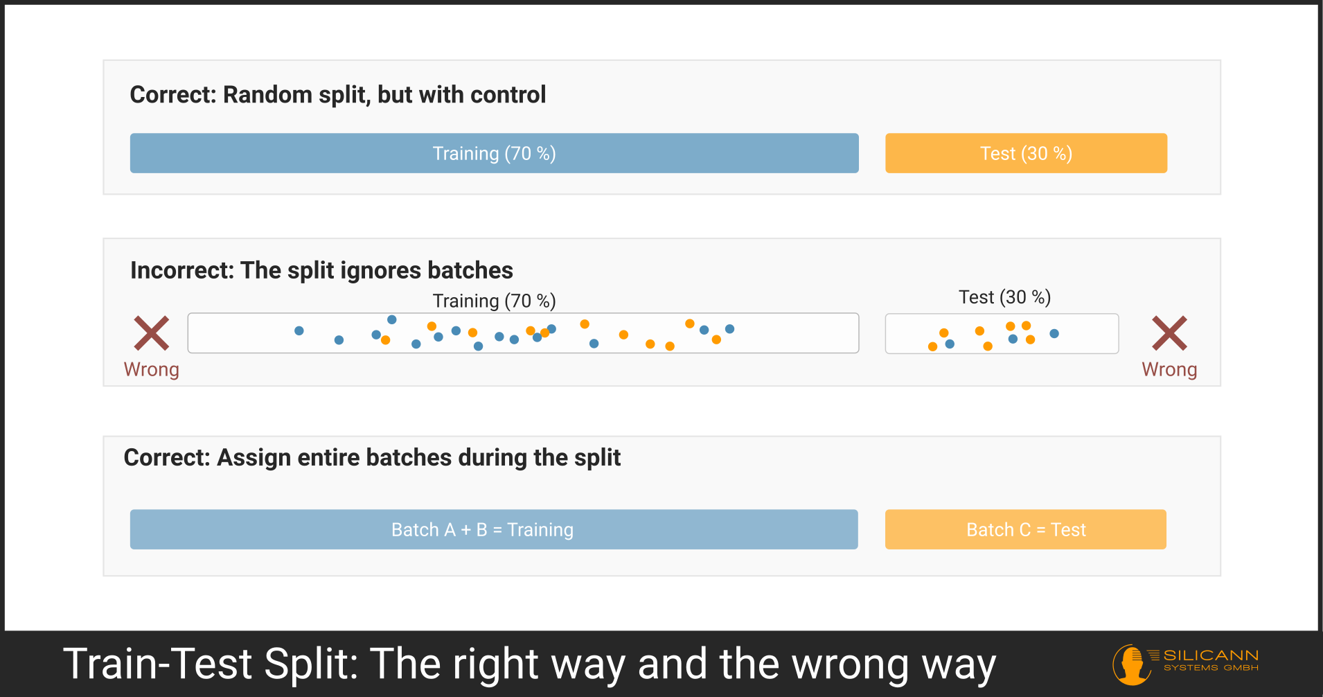
In such cases, one should either split in a stratified manner (e.g. with StratifiedShuffleSplit by concentration classes) or deliberately hold back entire batches for the test set. The goal is always that the test set reflects the later reality as realistically as possible.
Cross-Validation: More Information from Limited Data
The trade-off when splitting into training and test sets is that a significant portion of the samples lies idle in the test set. Especially with small datasets, this leaves little material for training. Additionally, the result depends on the randomness of the split - a different random_state can lead to noticeably different evaluations.
Cross-validation (CV) solves both problems. Instead of a single split, the dataset is divided into \(k\) equal-sized parts ("folds"). The model is trained \(k\) times, with a different fold serving as the test set each time and the remaining \(k-1\) folds handling the training. At the end, you have \(k\) independent evaluations, which are combined into an average (e.g. RMSECV - Root Mean Square Error of Cross-Validation).
from sklearn.model_selection import cross_val_score, KFold
from sklearn.cross_decomposition import PLSRegression

pls = PLSRegression(n_components=5)
kfold = KFold(n_splits=5, shuffle=True, random_state=42)

# cross_val_score uses R^2 (coefficient of determination) by default
scores = cross_val_score(pls, spectra, reference_values, cv=kfold, scoring='neg_root_mean_squared_error')
rmsecv = -scores.mean()
A special case of cross-validation is Leave-One-Out (LOOCV). Here, \(k\) equals the number of samples: each individual sample is used once as the test set, and all the others serve as training. The advantage is that nearly all data is used for every training run. The disadvantage: LOOCV is computationally intensive (with \(n\) samples, the model is trained \(n\) times) and can lead to optimistic estimates with highly correlated spectra because leaving out a single sample barely changes the spectrum. In most cases, 5-fold or 10-fold cross-validation is the better compromise between stability and computation time.
Unlike a simple train-test split, cross-validation delivers not just a single error figure but also provides information about the dispersion of model quality. An RMSECV of \(0.12 \pm 0.05\) tells a different story than one of \(0.12 \pm 0.01\) - in the first case, the model reacts sensitively to the specific data selection; in the second, it is robust.
RMSEC and RMSEP: The Two Numbers That Reveal Everything
Two error metrics stand at the centre of every model evaluation, and their relationship to each other is more informative than either one alone:
-
RMSEC (Root Mean Square Error of Calibration) describes the error the model makes on the exact data it was trained on. It becomes smaller with each additional PLS factor simply because the model gets more degrees of freedom to adapt to the training data. RMSEC does not capture whether what was learned is physically meaningful or just noise.
-
RMSEP (Root Mean Square Error of Prediction) is calculated on the independent test set, which was never part of the training. A low RMSEP means: the model generalises.
We can assess the quality of the model by looking at the difference between RMSEC and RMSEP:
| PLS Factors | RMSEC (Training) | RMSECV (Cross-Val.) | RMSEP (Test Set) | Interpretation |
|---|---|---|---|---|
| 2 | 0.45 | 0.48 | 0.47 | Underfitting, too few factors |
| 4 | 0.28 | 0.30 | 0.30 | Balanced, good generalisation |
| 6 | 0.18 | 0.31 | 0.34 | Beginning overfitting |
| 9 | 0.08 | 0.40 | 0.52 | Severe overfitting |
As long as RMSECV and RMSEP remain in the same order of magnitude, the model is learning genuine chemical relationships. However, when the RMSECV rises significantly above the RMSEC and the RMSEP deviates even further, overfitting has set in. In that case, the model is no longer describing the chemistry but rather its own training dataset.
from sklearn.metrics import mean_squared_error
import numpy as np

# Calibration on training data
pls.fit(X_train, y_train)
y_cal = pls.predict(X_train)
rmsec = np.sqrt(mean_squared_error(y_train, y_cal))

# Prediction on test data
y_pred = pls.predict(X_test)
rmsep = np.sqrt(mean_squared_error(y_test, y_pred))

print(f"RMSEC: {rmsec:.3f}, RMSEP: {rmsep:.3f}")
The Overfitting Trap
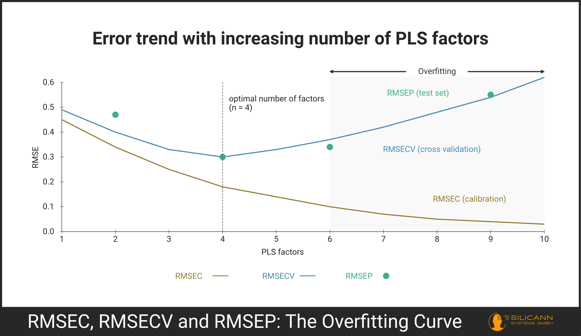
Overfitting is the most common and at the same time the most difficult to detect error when building chemometric models, because the model delivers excellent results at first glance. An \(R^2\) of 0.999 on the training set sounds like success. But it can also mean that the model has replicated every tiny fluctuation in the training dataset: detector noise, slight temperature drifts during measurement, inhomogeneities in individual samples. None of that is chemical information; it is chance, and on new samples, chance will look different. The prediction collapses.
A helpful analogy is the difference between understanding and rote memorisation. A model that has understood the relationships between spectral features and the target variable can transfer that knowledge to new spectra. A model that has memorised the answer key of its training data fails at its first transfer task.
In PLS regressions, overfitting typically appears as the RMSECV curve rising again after a minimum, while the RMSEC curve continues to fall monotonically. The optimal number of factors is at the minimum of the RMSECV, not where the RMSEC is lowest. A common mistake: choosing the number of factors to minimise calibration error, overlooking the fact that predictive ability was sacrificed long ago.
Train-Test Split or Cross-Validation? A Decision Guide
Both methods are tools for validation, but they solve different problems and are suited to different situations.
A single train-test split is the method of choice when sufficient data is available (in spectroscopic practice, from about 100-150 independent samples onward). It is simple to implement, quick to evaluate, and the held-back test set provides an honest, unbiased assessment. Moreover, it is the only validated statement of how the model will perform in later routine operation - because there, too, it encounters data it has never seen.
Cross-validation is the right tool whenever the number of samples is limited. It also helps with model optimisation: during development and when tuning hyperparameters (such as the number of PLS factors or the choice of preprocessing), cross-validation is used to compare different model variants without touching the test set. Only once the final model configuration is settled is the test set used - once.
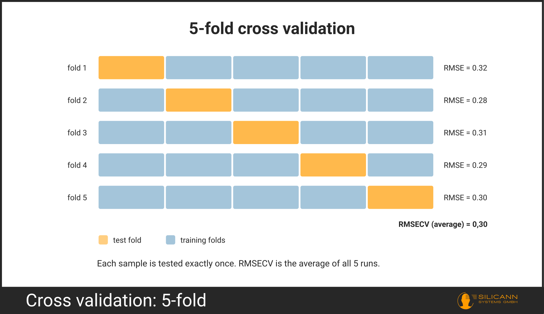
The ideal strategy for spectroscopic practice combines both approaches:
- Split the data: 70-80% training data, 20-30% test data.
- The test data is locked away and not touched until the very end.
- The model is developed on the training data: optimise preprocessing, select the number of factors, optionally select variable ranges. All evaluated exclusively with cross-validation on the training set.
- Only once the final model is settled is it evaluated once on the test set. The result is the RMSEP - and it is this figure that is communicated, not the RMSEC or RMSECV.
The Complete Workflow at a Glance
-
Data collection: Acquire spectra and reference values. Ensure diversity in the dataset (different batches, measurement days, concentration ranges); otherwise, the model will later learn only a slice of reality.
-
Preprocessing: Smoothing, derivatives, scatter correction (SNV, MSC) - depending on the application. Preprocessing is applied to the entire dataset before it is split. Crucially, it is parameterised on the training data and then applied identically to the test data.
-
Splitting: Separate data into training and test sets (70:30 or 80:20). If batch effects or repeated measurements are present or could be present, assign entire batches or measurement days as blocks.
-
Calibration with cross-validation: Build the model on the training set using \(k\)-fold cross-validation. Choose the number of factors at the minimum of the RMSECV curve, not at the minimum of the RMSEC.
-
Validation on the test set: Apply the finished model to the test set. Calculate RMSEP and compare it with RMSECV. If RMSEP and RMSECV are of the same order of magnitude, the model is trustworthy. An RMSEP significantly above the RMSECV indicates overfitting or a non-representative test set.
-
Routine operation: The validated model is put into daily measurement routine. Important: check at regular intervals with new reference samples whether the model is drifting - for instance because the sample matrix changes gradually or the spectrometer ages.
If these steps are followed, the result will be models that not only look good on paper but will also prove themselves when deployed in production.
| Feature | Spektralwerk 15 Core NIR |
|---|---|
| Wavelength range | 900-1700 nm |
| Detector array | InGaAs, 256 pixels |
| Signal-to-noise ratio (SNR) | up to 10000:1 |
| Sample rate / spectra per second | > 500 Hz (streaming mode) |
| Trigger in and trigger out | yes |
| Spectral resolution (FWHM) | 3.9 nm (Hg line at 1014 nm) 5 nm (Hg line at 1529.6 nm) |
| Interfaces | Ethernet, FC (SMA on request) |
| Operating temperature | -5°C to +30°C |
| Ingress protection | IP40 (higher on request) |
| Details | Learn more |
Looking for an NIR spectrometry solution?
Thank you for your message!
We will get back to you as soon as possible.
Unfortunately, we were unable to transmit your message.
A technical error occured. Please try again later — or send an email to sales@silicann.com.
Thank you for your understanding.